Intuition for maximal likelihood or posterior inference¶

Simple problem statement¶

Approximate a “parameter” \(\theta\), the average power of a brain signal.

Given:

Some power data \(y_i\), an imperfect realization of this signal
\(\theta\) is normally distributed

Consider:

\(\theta\) has a true value in principle, but it’s inaccessible to us.
The best we can hope to learn is a distribution \(p(\theta)\) of its values.
The peak of this distribution is our best bet.

_{Note 1: I am leaving out any discussion of priors}

_{Note 2: \(\theta\) has no relationship to any Fourier frequency bands}

An analogy¶

Imagine:

You are a hiker on a broad hill of \(\theta\) with no map
You are looking for its peak

What kind of device would be useful?

Some theory¶

Probability distribution for a normal variable is: normal

\[p(\theta) \sim {\rm exp}(-\frac{1}{2 \sigma^2}(y_i -\sigma)^2)\]

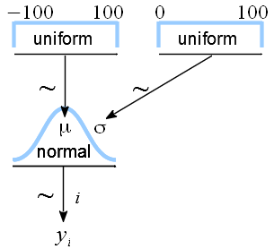
That’s the likelihood of \(\theta\) given our data.

Suppose we know \(\sigma\). Can we calculate \(\theta\) for a given \(y_i\)?

Approach 1: Maximum likelihood¶

To find the peak, simply follow “altimeter” up to find maximum likelihood (ML).

What’s at the peak?

That’s how linear mixed effects models are estimated: ML or REML.

Approach 2: Walking around and keeping score (eg Metropolis; used in Bayes)¶

Now imagine:

You are a hiker on a broad hill of \(\theta\) with no map
You are making a map

What kind of devices would be useful?

For each step you take:

Go to a location
Look at the altimeter (plug in data to equation)
Write down altitude (probability) and go to a new location

Ensure you visit every relevant location. One solution: https://chi-feng.github.io/mcmc-demo/app.html?algorithm=HamiltonianMC&target=banana

\[y_i = \alpha_{j[i]} + \beta x_{i} + \epsilon_i\]

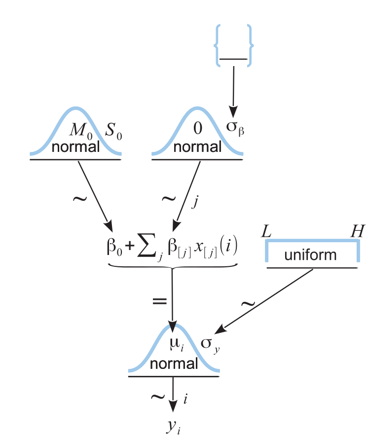
where:

\(j\) is mouse index
\(i\) is observation index
\(y_i\) is observed power
\(x_i\) is 0 (no stimulation) or 1 (stimulation)
\(\epsilon_i \sim \mathcal{N}(0, \sigma_y^2)\), error
\(\alpha_{j[i]} \sim \mathcal{N}(\mu_{\alpha}, \sigma_{\alpha}^2)\), random intercept
\( \beta \sim \mathcal{N}(?, ?)\) slope. We want to estimate its distribution

Note: this is not a sampling distribution (aka likelihood). We’d have to rearrange terms and substitute \(p(\theta) \sim {\rm exp}(-\frac{1}{2 \sigma^2}(y_i -\sigma)^2)\) for each \( \mathcal{N}(0, \sigma_y^2)\). That’s beyound our scope

Super complicated regression example¶

hierarchical

Complication 2: Integrate prior knowledge¶

Most often, numerical stability reasons and common sense information. For instance:

mountain height cannot be negative
its width is broad but finite

\[p(\theta|y_i) ~ p(y_i|\theta) {\bf p(\theta)}\]

_{(plus denominator, it’s not strictly relevant)}

Say \(p(\theta)\sim \mathcal{N}(0,100)\).

We’ll simply multiply by \(\mathcal{N}(0,100)\) for each step in sampling

Bayes-window examples

Intuition for maximal likelihood or posterior inference

Contents